There are following categories of handover (also referred to as handoff):
Hard handover means that all the old radio links in the UE are removed before the new radio links are established. Hard handover can be seamless or non-seamless. Seamless hard handover means that the handover is not perceptible to the user. In practice a handover that requires a change of the carrier frequency (inter-frequency handover) is always performed as hard handover.
Soft handover means that the radio links are added and removed in a way that the UE always keeps at least one radio link to the UTRAN. Soft handover is performed by means of macro diversity, which refers to the condition that several radio links are active at the same time. Normally soft handover can be used when cells operated on the same frequency are changed.
Softer handover is a special case of soft handover where the radio links that are added and removed belong to the same Node B (i.e. the site of co-located base stations from which several sector-cells are served. In softer handover, macro diversity with maximum ratio combining can be performed in the Node B, whereas generally in soft handover on the downlink, macro diversity with selection combining is applied. Generally we can distinguish between intra-cell handover and inter-cell handover. For UMTS the following types of handover are specified: The most obvious cause for performing a handover is that due to its movement a user can be served in another cell more efficiently (like less power emission, less interference). It may however also be performed for other reasons such as system load control. The different types of air interface measurements are: The UE supports a number of measurements running in parallel. The UE also supports that each measurement is controlled and reported independently of every other measurement. Further reading: 3GPP 25.331 |
Further reading: 3GPP TS 25.303, 25.331
During the cell search, the UE searches for a cell and determines the downlink scrambling code and frame synchronisation of that cell. The cell search is typically carried out in three steps:
Step 1: Slot synchronisation
During the first step of the cell search procedure the UE uses the SCH's primary synchronisation code to acquire slot synchronisation to a cell. This is typically done with a single matched filter (or any similar device) matched to the primary synchronisation code which is common to all cells. The slot timing of the cell can be obtained by detecting peaks in the matched filter output.
Step 2: Frame synchronisation and code-group identification
During the second step of the cell search procedure, the UE uses the SCH's secondary synchronisation code to find frame synchronisation and identify the code group of the cell found in the first step. This is done by correlating the received signal with all possible secondary synchronisation code sequences, and identifying the maximum correlation value. Since the cyclic shifts of the sequences are unique the code group as well as the frame synchronisation is determined.
Step 3: Scrambling-code identification
During the third and last step of the cell search procedure, the UE determines the exact primary scrambling code used by the found cell. The primary scrambling code is typically identified through symbol-by-symbol correlation over the CPICH with all codes within the code group identified in the second step. After the primary scrambling code has been identified, the Primary CCPCH can be detected and the system- and cell specific BCH information can be read.
If the UE has received information about which scrambling codes to search for, steps 2 and 3 above can be simplified
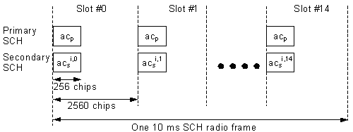
The Synchronisation Channel (SCH) is a downlink signal used for cell search. The SCH consists of two sub channels, the Primary and Secondary SCH. The 10 ms radio frames of the Primary and Secondary SCH are divided into 15 slots, each of length 2560 chips. Picture above illustrates the structure of the SCH radio frame.
The Primary SCH consists of a modulated code of length 256 chips, the primary synchronization code (PSC) is transmitted once every slot. The PSC is the same for every cell in the system.
The Secondary SCH consists of repeatedly transmitting a length 15 sequence of modulated codes of length 256 chips, the Secondary Synchronisation Codes (SSC), transmitted in parallel with the Primary SCH. The SSC is denoted csi,k in figure 20, where i = 0, 1, …, 63 is the number of the scrambling code group, and k = 0, 1, …, 14 is the slot number. Each SSC is chosen from a set of 16 different codes of length 256. This sequence on the Secondary SCH indicates which of the code groups the cell's downlink scrambling code belongs to.
Summary of the process:
| Channel | Synchronisation acquired | Note |
| Primary SCH | Chip, Slot, Symbol Synchronisation | 256 chips The same in all cells |
| Secondary SCH | Frame Synchronisation, Code Group (one of 64) | 15-code sequence of secondary synchronisation codes. There are 16 secondary synchronisation codes. There are 64 S-SCH sequences corresponding to the 64 scrambling code groups 256 chips, different for different cells and slot intervals |
| Common Pilot CH | Scrambling code (one of 8) | To find the primary scrambling code from common pilot CH |
| PCCPCH *) | Super Frame Synchronisation, BCCH info | Fixed 30 kbps channel 27 kbps rate spreading factor 256 |
| SCCPCH **) | | Carries FACH and PCH channels Variable bit rate |
*) Primary Common Control Physical Channel
**) Secondary Common Control Physical Channel
Further reading: 3GPP TS 25.211 25.213
High Speed Downlink Packet Access (HSDPA) is a packet-based data service in W-CDMA downlink with data transmission up to 8-10 Mbps (and 20 Mbps for MIMO systems) over a 5MHz bandwidth in WCDMA downlink. HSDPA implementations includes Adaptive Modulation and Coding (AMC), Multiple-Input Multiple-Output (MIMO), Hybrid Automatic Request (HARQ), fast cell search, and advanced receiver design.
In 3rd generation partnership project (3GPP) standards, Release 4 specifications provide efficient IP support enabling provision of services through an all-IP core network and Release 5 specifications focus on HSDPA to provide data rates up to approximately 10 Mbps to support packet-based multimedia services. MIMO systems are the work item in Release 6 specifications, which will support even higher data transmission rates up to 20 Mbps. HSDPA is evolved from and backward compatible with Release 99 WCDMA systems.
Currently (2002) 3GPP is undertaking a feasibility study on high-speed downlink packet access.
 |
Further reading:
3GPP TS 25.855 High Speed Downlink Packet Access (HSDPA); Overall UTRAN description
3GPP TS 25.856 High Speed Downlink Packet Access (HSDPA); Layer 2 and 3 aspects
3GPP TS 25.876 Multiple-Input Multiple-Output Antenna Processing for HSDPA
3GPP TS 25.877 High Speed Downlink Packet Access (HSDPA) - Iub/Iur Protocol Aspects
3GPP TS 25.890 High Speed Downlink Packet Access (HSDPA); User Equipment (UE) radio transmission and reception (FDD)
 |
TDD WCDMA uses spreading factors 4 - 512 to spread the base band data over ~5MHz band. Spreading factor in dBs indicates the process gain. Spreading factor 128 = 21 dB process gain). Interference margin is calculated from that:
Interference Margin = Process Gain - (Required SNR + System Losses)
Overview of Spreading Process |
WiMAX Forum RF Network Engineer Certification Training Material Chapter 3, Antennas for WiMAX
0 comments Posted by communications at 7:37 PMAfter the first and second chapter of my self learning, here we go the third chapter ![]() titled Antennas for WiMAX. Just like traditional Wireless System, there are 3 kinds of antenna used for transceiving Radio Access Signal i.e., Omnidirectional, Sectoral, and Point to Point. The use of those antenna depends on it’s application.
titled Antennas for WiMAX. Just like traditional Wireless System, there are 3 kinds of antenna used for transceiving Radio Access Signal i.e., Omnidirectional, Sectoral, and Point to Point. The use of those antenna depends on it’s application.

1. Omnidirectional, broadcast 360 degree suitable for large area rural environment.

2. Sectoral, broadcast on intended area: 60, 90, and 120 degree. This kind of antenna is suitable for urban environment which has lage population on a certain area.

3. Point to Point Antenna is used for point to point communication, i.e., Microwave link, backbone etc.

(pictures are filched from wimax.com). If you need to read WiMAX Application material, please visit this my previous post, here
After we have discussed about those traditional antennas, now we are going to discuss advanced antenna technology in WiMAX.
1. Antenna Diversity,
Using two or more receiving antennas on a wireless device to eliminate multipath signal distortion. Typically, the signal from the antenna with the least noise (best SNR) is chosen, and the other antenna is ignored.
There are three techniques in diversity scheme:
1. Space Time Coding (Alamouti Code), is a method employed to improve the reliability of data transmission in wireless communication systems using multiple transmit antennas. STCs rely on transmitting multiple, redundantcopies of a data stream to the receiver in the hope that at least some of them may survive the physical pathbetween transmission and reception in a good enough state to allow reliable decoding. (resource: http://en.wikipedia.org/wiki/Space–time_code) Space time codes may be split into two main types:
- Space–time trellis codes (STTCs)[1] distribute a trellis codediversity gain. over multiple antennas and multiple time-slots and provide both coding gain and
- Space–time block codes (STBCs)[2][3] act on a block of data at once (similarly to block codes) and provide only diversity gain, but are much less complex in implementation terms than STTCs.


 .
.This is my first Chapter on my own WiMAX RF Engineer self learn. As I mentioned before in my post this first chapter contains Module 1material:
6 WiMAX Applications (after walking around the web, I found an interesting material from Intel)
 On the picture above there are 6 applications and it’s architecture which is grouped in to three items:
1. Access (Appropriate standards: 802.16d-2004 and 802.16e)
- Fixed Outdoor
- Backhaul
2. Portability (Appropriate standard: 802.16e)
- Nomadic Metrozone
- Fixed Indoor
- Enterprise, Campus Piconet
3. Mobility
- Mobile Application
Standards Specification

Spectrum availability, there are two kind of spectrum frequency:
- Licensed Spectrum
- Unlicensed Spectrum

-
- From picture above we can conclude, WiMax Main RF Bands are: 2.3 GHz, 2.4 GHz, 2.5 GHz, 3.5GHz, 5.8 GHz, and (maybe) 700 GHz.
802.16e Standard Enhancement.
First WiMax standard was published in April 2001 and completed in October 2001. And as amendment 802.16a was approved in 2003. After 2003 the standard development continuous and breed 802.16d in 2004. And then in 2005, 802.16e was approved and add the mobility to the standard.
So what is the different between 802.16d and 802.16e? Well… let me show you what I’ve got ![]()
- 802.16d
- NLOS application and indoor CPE are supported.
- Beam forming Antenna
- OFDM Subchannelization
- FBWA Technology (wireless DSL Alternative)
- 802.16e (called “Mobile WiMax)
- Supports Portable BWA
- Operated on 2.3 GHz, 2.5 GHz and 6 GHz
- Handoff and Roaming Support
- Scalable OFDMA, OFDMA with subchannelizatoin
From the brief introduction above, we can conclude that 802.16e enhancement is about mobility, as we can see it supports Portable BWA, Handoff and Roaming.
As I am studying WiMAX RF Technology now, the tittle above is my certification wish list ( I hope I can take it… ![]() ). While I’m dreaming about this kind of certification, I do some web walking and find this Certification syllabus:
). While I’m dreaming about this kind of certification, I do some web walking and find this Certification syllabus:
WiMAX Forum RF Network Engineer Certification™
Module 1: WiMAX Network Design Options
- List six applications of WiMAX technology
- Match each application to its WiMAX specification, frequency band, and architecture
- Describe five 802.16e mobile WiMAX enhancements
Module 2: Review of RF Fundamentals
- Calculate power levels in dBm, Watts and ìV/m
- Apply Nyquist and Shannon observations to calculations of the bandwidth of channels, and to WiMAX’s adaptive modulation and coding
Module 3: Antennas for WiMAX
- List three antenna diversity techniques
- Describe the operations of two types of MIMO systems and two types of Advanced Antenna Systems
Module 4: RF Design Considerations for WiMAX
- Describe the sources of noise based on bandwidth and operating frequency
- Determine the system noise floor based on bandwidth and Noise Figure
- Determine system performance based on C/N and Eb/No
Module 5: Performing a WiMAX Link Budget
- Determine LOS and NLOS Maximum Allowable Path Loss (MAPL) based on system parameters
- Determine power settings for a balanced path
- Use spreadsheets to design for specified lognormal fading probability
- Perform a link budget based on manufacturer’s equipment parameters and system requirements
Module 6: WiMAX Path Loss Modeling
- Determine expected point-to-point link performance using an analytical path loss model
- Calculate expected NLOS performance using an empirical path loss model
- Determine the amount of margin required, based on lognormal fading
Module 7: Frequency Reuse in Fixed and Mobile WiMAX Networks
- Design the frequency reuse plan for your WiMAX network, working with your equipment vendor
- Diagram FUSC and PUSC permutation zones
- Discuss several reuse proposals for mobile WiMAX networks
Module 8: WiMAX Performance and Coverage Considerations
- Explain and follow each step of the WiMAX Three- Phase Network Design process
- List eight WiMAX-specific network design considerations
- Model a flat-earth WiMAX network with the Design spreadsheet, and determine sensitivity of the estimated economic payback to changes in market and technical factors
- Determine site selection criteria
- Determine cell density required for a desired level of service, performance, and coverage.
- Choose backhaul options to support throughput requirements
Module 9: WiMAX Coverage and Performance Planning with modeling tools
- Employ a modeling tool to prepare an RF plan for your network in a three-part case study
- Illustrate the effect of frequency, power, terrain, clutter and CPE location on coverage
- Import terrain and clutter databases
- List options for accommodating system and subscriber growth
Module 10: Capacity Design, and Oversubscription
- Mathematically relate oversubscription and subscriber quality of service
- Validate vendor design rules for capacity planning
Wow.. what a wonderful training materials. But the most sophisticated is, we have an opportunity to get WiMAX Forum RF Engineer Certificate. I have to plan another saving to this Certification ![]() Ganbatte!
Ganbatte!

Europe UK : Sensustech has launched Insight 3G, an automated monitoring system for 3G and EDGE network service availability and data services performance. The system uses compact automated measurement devices called “Performance Analysis Mobiles” or “PAMs” fitted to vehicles that are moving around the network anyway such as buses, taxis and delivery vehicles. This automated approach, claims the company, allows the collection of as much as 30 times more measurements by comparison with traditional “drive test” approaches to quality measurement.
3G data collected includes 3G coverage and availability, session establishment attempts and any failure reasons, session establishment time, up and downlink transmission rates, data latency and error rates for up and downlink data. These data elements can be reported in a variety of ways: Insight Geographical Information System (GIS) distribution of data, trends, comparisons between competing networks and achievement against key performance indicators
Says Sensustech’s Head of Marketing, Robin Burton: “We believe that effective network management can only be achieved if sufficient, statistically significant, information is available on delivered network quality. The dynamic nature of 3G coverage means that many more measurements are needed by comparison with 2G networks. Insight 3G allows executives to have a view of delivered quality, across the network, from day to day and at different times of the day.”
Says Brian Lancaster, Sensustech Technical Support Manager: “3G PAMs use an integral wireless module to provide data backhaul as well as the ability to simultaneously monitor delivered GSM or GPRS voice and data performance. 3G performance is monitored either via an integrated 3G module or via an adjunct 3G handset. This allows us to provide a standardised view of delivered quality across the network and to offer an assessment of the quality delivered by a variety of WCDMA, IS-95, CDMA-2000 and EDGE handsets. .”
The Sensustech Insight system delivers reports of vital interest to strategic management, sales and marketing teams, roaming management, network management, investors, corporate users of mobile communications and industry regulators.
About Sensustech
Sensustech is borne from a core team of network operational and technical managers that has been working together for more than 15 years. During that time they have worked with virtually every major operator around the world on high availability and network engineering projects.
Sensustech is an AlanDick company.
The AlanDick Group of companies is a total solutions provider with the global logistics capability unique in its ability to provide innovative products and services to satisfy the communication network infrastructure needs of cellular, broadcast, radar/surveillance & enterprise markets.
With 41 offices across 5 continents AlanDick is a world leading organisation with the ability to plan, design, deploy, develop, maintain, manage, support, integrate & optimise communication networks across the globe.
High Speed Downlink Packet Access (HSDPA) is a packet-based data service in W-CDMA downlink with data transmission up to 8-10 Mbps (and 20 Mbps for MIMO systems) over a 5MHz bandwidth in WCDMA downlink. HSDPA implementations includes Adaptive Modulation and Coding (AMC), Multiple-Input Multiple-Output (MIMO), Hybrid Automatic Request (HARQ), fast cell search, and advanced receiver design.
In 3rd generation partnership project (3GPP) standards, Release 4 specifications provide efficient IP support enabling provision of services through an all-IP core network and Release 5 specifications focus on HSDPA to provide data rates up to approximately 10 Mbps to support packet-based multimedia services. MIMO systems are the work item in Release 6 specifications, which will support even higher data transmission rates up to 20 Mbps. HSDPA is evolved from and backward compatible with Release 99 WCDMA systems.
Currently (2002) 3GPP is undertaking a feasibility study on high-speed downlink packet access.
|
In this post, I’ll try to share about my experience in Cellular Radio Network Optimization. This post consists of several subject that maybe useful to upgrade our knowledge and I well opened if there are questions relate to those subject. Please feel free to discuss with me, you can post it on comment or send email.
Why Optimization?
Below, I’ll mention optimization objectives generally,
- increasing network availability (deal with call performances, i.e., drop calls reduction to increase the access completion rates, handover control : assure enough handover to cover costumers mobility)
- increasing network quality (deal with speech and data quality to increase customer satisfaction)
- increasing network capacity (deal with capacity management efficiently, i.e., maintaining network resources to meet customer base needs so the blocking possibility is minimum)
n
n
well… after we’ve talked about optimization aims, below we’ll discuss about optimization
procedures. First, we need to know how’s the network developmnt process takes place. After Radio Network Planning Process and network are being implemented, Radio Tuning (a.k.a basic radio optimization) and Radio Verification have to be done to assure that the network meet the operator needs. And, after Operator have accepted the network and network UP here we go..the (extended) Optimization process is begin.
Radio Optimization is done because several causes,
- systematics inacurracies (Tool database, prediction algorithms..)
- statistical processes involved (Radio Propagation, traffic..)
- Assumption made
- Human error (Planning errors, data entry, installation errors…)
- equipment faults (hardware and software)
- network growth
causes that mentioned above, could make network anomaly and it influence the customer satisfactions. So… from costumer complains statistics we know where and when does the
network unstability take a place. Hmm…is there any left behind?? yup… we have to know what, why, and how…We need The (extended) radio Optimization to answer thoose question’s left, so we can cure the network unstability ^_^
From the description above, we can conclude that Optimization process is devided into Basic Radio Optimization and Extended Radio Optimization. Both of them are controled by O&M(Operation and Maintenance). The main difference is that the Basic Radio Optimization will be done before network launch, and Extended Radio Optimization will be done after network is launched with normal subscriber.
2. Basic Radio Optimization (Radio Tuning)
System Tuning is done on this process, in order to meet the Operator requirements. The tuning activity have to change several cell paramaters, so the quality requirement is reached. On the high coverage and traffic demands areas usually this processes will be repeated a number of times untill the system reach Optimum performance.
3. Extended Radio Optimization
This process is done as customer complains follow-up. In the real network which is loaded by customer’s traffic, it often suffer several problems that effect the customer satisfaction. From customer complains statistics we can locate the network problem and when did it took a place. After we know where and when, the Optimization team will go to that spot and do tests measurement to take a log file and check the equipment conditions.
The tests measurement and equipment conditions data will be analyzed to make recommendation so the network problem can be fixed.
4. Tests Measurements
This activity is carried out with test mobile system (i.e., laptop with tests measurement software installed, Mobile station, and GPS for outdoor case) to record logfile that contains the signaling information send over the air interface and will consists following paramaters:
- Information for channel in use (serving cell):
BCCH
ARFCN
BSIC
TIMING ADVANCE
TX POWER (MS)
RX Qual
RX Lev
- Information for handover candidates (neighbors cell)
BCCH
BSIC
RxLev
note : on my projects, I use TEMS investigation 4 or above..
Hmm.. before we go to the next subject, we have to know the deffinition of paramaters which is mentioned above. ^_^
BCCH : Broadcast Control Channel is a key channel contains information about network configuration (network to MS direction) which is used for neighbouring cell measurements to determine cell reselections and handovers. BCCH allocation (BA) is a list of BCCH carriers in use within a specific geographical area of PLMN. It Indicates the RF Channels that the MS required to monitor while camped on a cell of that PLMN. BCCH term’s frequently used to refer to a carrier or a channel that often lead to confusion. Well on this case, it means carrier or channel.
ARFCN : Absolute radio frequency channel number. An identifier or number of a channel used on the Air-interface. From the ARFCN, it is possible to calculate the frequency of the uplink and the downlink that the channel uses.
BSIC :Base station identity code. An identifier for a BTS, although the BSIC does not uniquely identify a single BTS, since it has to be reused several times per PLMN. The purpose of the BSIC is to allow the mobile station to identify and distinguish among neighbor cells, even when neighbor cells use the same BCCH frequency. Because the
BSIC is broadcast within the synchronization channel (SCH) of a BTS, the mobile station does not even have to establish a connection to a BTS to retrieve the BSIC. It consists of the network color code (NCC), which identifies the PLMN, and the base station color code (BCC).
TA : Timing advance. The agreement in a GSM system is for the MS to send its data three time slots after it received the data from the BTS. The BTS then expects the bursts from the MS in a well-defined time frame. This prevents collision with data from other mobile stations. The mechanism works fine, as long as the distance between MS and BTS is rather small. Increasing distance requires taking into account the propagation delay of downlink bursts and uplink bursts. Consequently, the mobile station needs to transmit earlier than defined by the “three time slots delay” rule. The information about how much earlier a burst has to be sent is conveyed to the mobile station by the TA. The TA is dynamic and changes in time. Its current value is sent to the mobile station within the layer 1 header of each SACCH. In the opposite direction, the BTS sends the current value for TA within the MEAS_RES messages to the BSC (e.g., for handover consideration). The farther the MS is away from the BTS, the larger is the required TA. Using the TA allows the BTS to receive the bursts from a particular MS in the proper receiver window. The BTS calculates the first TA when receiving a RACH and reports the value to the BSC. TA can take any value between 0 and 63, which relates to a distance between 0 km and 35 km. The steps are about 550 m (35 km/63 » 550 m). With respect to time, the different values of TA refer to the interval 0 ms through 232 ms, in steps of 48/13 ms. It is important to note that this value of TA represents twice the propagation delay.
Tx Power (MS): Power transmited by Mobile Station
RxLev: RXLev provides the results of the measurement of the receiving level on the
Air-interface. These measurements are performed independently by the MS and the BTS. On this case RxLev is measured on the MS.
RxQual : RXQUAL values, are relevant for the decision of a BSC on power control and handover. They indicate the bit error rate that was measured on the Air-interface. The bit error rate can be determined by facilitating the training sequence. If you want to learn more… you can read the gsm recommendation
Measurements are to be taken on request from the analyzing team due to prioritizing form the coordinator. The data collection will partly consist of pure measurements and a pre analysis of the collected data.
Data collection can be divided in to three parts:
- continuous drive test (drive over an area to detect poor coverage, handover missed, interference..etc)
- spot drive test (dedicated measurement on specific problem spots for detail analyzing of particular problem)
- network performance test (typical measurements over a hugh area i.e., town or road distance, such as: Call Success Test, Quality level, etc.)
Should be noted that after each data collecting, the docummentation of data results must be regulated nicely, so on the post processing the analyze team can use that results easily.
well…if there’s no question, I’ll go to the next subject. :p
5. Measurement Analysis
The main goal of Optimization process is to improve the network performance. This is the list of analysis :
- signal strength (is checked according specified mobile classes inside actual coverage area)
- adjacent and cochannel interference
- handover pattern (to avoid “Ping Pong” handover)
The results of these analysis is Technical Recommendation wich is deal with action request for equipment config change both hardware (antenna configuration,etc.) and software (RF parameters).
n
I think is enough for this post, I’m afraid it’s too theoretically :P. Hmm.. maybe on the next chapter.. I’ll post a little bit “practical”, about tools, about TEMS, about hardware, about post processing, etc. Just wait and see…
First I’d like to show you the network architecture that I filched from www.ccpu.com:

On the network architecture above, we can see 4G(3G LTE/SAE), 3G/3.5G HSPA, and IMS convergence. It should be noted that the picture above implement backward compatibility technology i.e., 3GPP IMT 2000 and IMT advanced.
We know, beside 3GPP there’s another technology such as 3GPP2 (based on CDMA2000 evolution and UMB) and also WiMAX. So… how we choose the interoperability scenario for this various technology?
Below I give another picture from www.telkom.info, so we can distinguish the differences

hmm… is there any left behind? yup, we haven’t talked about WiMAX Network architecture yet. So below I post another picture related to WiMAX architecture:

Well, after we know each network architecture, now we will begin to discuss about the interoperability or interworking between them.
First of all, we have to equalize our perception about network architecture. Commonly, we can divide the network architecture into three main parts, i.e., Radio Access Network, Transmission Network ( Transport) and Core Network.
Well, after we have same perception about network architecture, now we can focus on Radio Access Network which is experienced rapid development in this 5 past years.
Hmm… as mentioned on Wikipedia, 4G objectives are:
- A spectrally efficient system (in bits/s/Hz and bits/s/Hz/site)
- High network capacity: more simultaneous users per cell,
- A nominal data rate of 100 Mbit/s while the client physically moves at high speeds relative to the station, and 1 Gbit/s while client and station are in relatively fixed positions as defined by the ITU-R,
- A data rate of at least 100 Mbit/s between any two points in the world,
for the points above, let’s take a look this picture:

what can we see on the picture above is: all the evolution are using OFDMA!! so we can conclude that 4G technology are seems to be OFDMA and it’s evolution using MIMO, MISO, beamforming, etc. in order to achieves high network efficiency, high network capactiy, high data rate ( though less than 100 Mbps ). In other word: LTE, UMB, and WiMAX just like a brother and sister huh..
- Smooth handoff across heterogeneous networks,
- Seamless connectivity and global roaming across multiple networks,
for this two point above, I have my own opinion: All the network which is standardized by 3GPP and 3GPP2 are based on wide area concept ( GSM, CDMA, 3G UMTS, LTE, UMB). So how about the other network such as PAN, WLAN, which is based on small area concept?? How we can make those network interwork each other? As we know that on 4G beside horizontal handover ( intrasystem handover ), 4G system should have vertical handover capability ( intersystem handover ) to get the network access in harmony with user application QOS. So… we have to build a hybrid network which can adopt wide area concept and small area concept in to one system. The alternative solution is to have Software Defined Radio on the User Equipment. With this kind of technology, smooth handover across heterogeneous system and global roaming across multiple networks can be achieved :D.
- High quality of service for next generation multimedia support (real time audio, high speed data, HDTV video content, mobile TV, etc)
- Interoperability with existing wireless standards, and
- An all IP, packet switched network.
hmm.. now we are going to discuss about the three last points. Well, as we have discussed above the most rapidly development technology is on the Radio Access side. But don’t forget, on 4G we have to maintain QOS for various application, over IP end to end network, without ignoring the interoperability with the existing wireless standards. So… what should we do??
Thanks god.. we have IMS. Yup!! the IP Multimedia Subsystem. With this element on the core network, what ever the radio access technology as long as it use IP, IMS can handle it. And don’t forget IPv6 to address all of equipment in this world…hehehe…
btw…jd inget slogan makanan : “Apapun makanannya, minumnya teh Botol Sosr*!!”, mungkin dalam dunia telekomunikasi… bisa kita ubah slogan tersebut menjadi: “Apapun teknologi akses radionya…core networknya: IMS!! ”
Well… maybe sometimes I’ll make an article about IMS… (after I’ve learned about it…). Thanks for the attention…hope this article will be useful. I’m sorry if there’s a lot of mistakes.. and I well opened to discuss it
In this post, I wanna share with you about CDMA2000 Optimization Procedure. Hope you’ll enjoy it!
Wireless network Optimization can be devided in to three layers:
- Device Layer
- Network Layer
- Resource Utilization Layer
We can conduct some methods to examine problems on those layers, i.e.,
- Drive tests and Analysis
- Signaling Tracking
- OMC analysis
- Synthesis
Let’s we go in to deep to each layer above,
- Device Layer
- Antenna and Feeder Cable Fault
- Transmission Fault
- GPS Fault
- Wireless Configuration
- Office Direction Problem
- Termination Problem
- Network Layer
- Solving Dropped Call Problem with Drive Test and Analysis Method
- Solving Problem with OMC Analysis Method
- Improving Coverage with Synthess Method
- Resource Utilization Layer
- Network Block Optimization
CDMA Performance Indicators
RF Performance indicators captured by drive-test activity. It show the CDMA RF environment to guide Optimization and Troubleshooting in air interface. Some parameters indicate uplink conditions, some downlink, and some both. These parameters collected at the subscriber side, so it’s easy to capture using commercial handset equipment without BSC’s assist.
Basic knowledge about CDMA spread spectrum signal characteristics such as: channel definitions, power control system, call processing flow, signal behaviour in noise and interference, and RF units ( transmitter and receiver) are needed, to analyse the parameters below.
- FER (Frame Error Rate) -> an excellent call quality summay statistic, it’s the end result of the whole transmission link
- reverse channel -> realized on the Base Station
- forward channel -> realized at handset
- if FER is good, any other problems aren’t having much effect
- if FER is bad, we have to check other indicators to analyze the network problem, because FER is just the end-result of the problem
- Mobile Receiver Power (Rx)-> Received Power at the handset (dBm). It should be noted that Received Power is Important, but it’s exact value isn’t critical.
- High Rx value (-35 dBm or higher) could cause overload condition in Amplifier sensitivity, intermod and code distortion on received CDMA signals.
- Low Rx value (-105 dBm or weaker would leave too much noise in the signal after de-spreading, resulting symbol errors, bit errors, bad FER and other problems.
- Ec/Io -> We can’t just use the handset’s power level to guide handoffs because it represents the total power measurement from all sectors reaching the handset. To measure the the signal level of each sector individually, we have to use each sector’s pilot (Walsh 0) as a test signal to guide handoffs.
- Ec/Io is a parameter, represents pilot cleannesses.
- foretells the readability of the associated traffic channels to guide soft handoffs decision
- derived from: ratio of good to bad energy seen by search correlator at the desired PN offset -> Ec/Io(forward) = Pilot Energy / (Paging + Synch + Traffic) Energy. Can be degraded by strong RF from other Cells, Sectors (imperfect PN orthogonality could cause -20 dB degradation) and also by noise.
- in Light condition (without traffic) Ec/Io = 3 dB, in Heavy loaded Ec/Io = -7 dB
- in a clean Situation which theres a sector dominant, Ec/Io just as good as it was when transmitted. But in “Pilot Pollution” condition, mobile hears a ’soup’ made up of all the overlapped sectors signal. So Io is the sum of all the signal received by MS, and Eo is the energy of desired sector’s Pilot signal. The Large Io will overrides the weak Ec -> Ec/Io is too Low!
- Handset Transmitter power (TxPO)
- TxPO is the actual RF power output of the handset transmitter(max= 23 dBm), including combined of open loop power control and closed loop power control (TxGA)
- this is the simple formula : TxPO = -(Rx dBm) - C + TxGA ( C= +73 for 800 MHz systems, and C=+76 for 1900 MHz systems) to reach balance link.
Maybe enough for this post.. because I have a low battery condition now :P, and I forgot to bring may laptop’s charger…
Hope this post useful for us…
The Data center Manager is responsible for computing, network communications, technical maintain and superiority assurance. The position involves and requires service delivery management and hands-on.
Data Center Manager (DCM) is an activity division software explanation. It facilitates revelation of your complete data center communications from the data center during the stand to procedure and mechanism within those procedures. Complete records are structure into the system for organization today's complex situation. Demonstration, and limitless "what if" situations are center elements of the software. Data Center Manager (DCM) presents the capability to study data in tabular and graphical layouts. Make conversant decisions; allow day to day efficiencies and procedures essential for positive Management of the data center with DCM.
Visualization presents a console display for a high level view of the DC. Selectable layers can be added to display power utilization, heat generation, current, and either power or signal port accessibility. Extra layers can be added to display door swings, hot cold aisles, position and density of perforated tiles, etc., to create truly customized displays.
Documentation offers apparent and expressive reporting on the IT communications. Customizable information element what assets are used and summarize per row and data center. Custom assets can be used to show how devices broadcast to acquiescence. Typical reports range from an assembly report that provides step by step instructions to assemble and cable a solution, to connectivity reports, power consumption, environmental reports, and asset management reports.
Modeling permits the clients to achieve unlimited "What if" scenarios. DCM swiftly decides the collision of data center consolidations, or the resource utilization associated with new data centers. The user can create detailed comparisons of planned apparatus upgrades against the present situation.
Analysis offers immediate contact to critical information and enables assessment making capability on key data center issues. Direct access to information such as accessibility of space, power, heat and cooling, port availability, and remaining weight capacity in racks, allows the user to make critical decisions with assurance.
Management capacities allow the user to organize and decommission devices rapidly and simply. Track apparatus through getting, staging, commissioning, decommissioning, and storage.
Detailed Responsibilities of DC Manager:
Control and make possible systems preservation for the following coordination: Fire Suppression; HVAC; Physical Security; Logical Security.
Own and supervise vendor relationships associated with co-location facilities where ACS has opted to situate utensils and/or services
Started methodology and guidelines for moving apparatus and services in and out of the DC capability
Enforce process for implementation modifies within the DC to include facilities, situation, customer tools, networking, etc.
Statement to administration on metrics connected with capability, topic remediation, preservation concerns, trending connected with all issues of success related to delivery of DC services, as well as customer connected concerns.
Improvement and completion of services required
Supervise and control physical safety for all DC properties and assets.
Radio Wave Propagation Models Used in RF Coverage Analysis
0 comments Posted by communications at 11:54 PMRadio wave propagation can be categorized as LOS (Line Of Sight) and non-LOS modes. LOS is direct point-to-point propagation with no obstructions in between. Non-LOS is indirect propagation in the absence of LOS path which consists of diffraction, reflection and scattering. In the HF band (3 - 30 MHz), propagation is primarily using sky wave for long distance communications. VHF and UHF (30 MHz - 3 GHz) waves travel by LOS and ground bounce propagation. The SHF (3 to 30 GHz) wave uses strictly LOS propagation.
The goal of propagation modeling is to determine the probability of satisfactory performance of a wireless system that depends on radio wave propagation. For RF systems planning, the modeling of propagation is for the purpose of RF coverage analysis. This analysis uses the propagation model and terrain data to predict the RF coverage area of a transmitter, the received signal strength at the end of a wireless link, the path loss from the transmitter to a distance receiver, the antenna tilt angle of the transmitter, the minimum antenna height to establish Line of Sight communication path and channel impairment such as delay spread due to multi-path fading.
Propagation models for different applications, environments and terrains had been developed by the US government, private organizations and standard body such as International Telecommunications Union (ITU). These models are based on large amount of empirical data collected for the purpose of characterizing propagation for that application. Since propagation models are created using statistical methods, no single model will exactly fit any particular application. It is a good idea to employ two or more independent models and use the results as bounds on the expected performance. The following are a list of most commonly used near-earth propagation models.
Longley-Rice
The Longley-Rice model predicts long term median transmission loss over irregular terrain. It is designed for frequency from 20 MHz to 20 GHz and path length from 1 to 2000 Km. The model accounts for terrain, climate, subsoil conditions and ground curvature. Longley-Rice model has two modes, point-to-point and area. The point-to-point mode uses detail terrain data and characteristics to predict path loss, whereas the area mode uses general information about the terrain characteristics to predict path loss.
Okumura
The Okumura model is based on the measurements made in Tokyo in 1960, between 200 to 1920 MHz. The measured values are used to determine the median field strength and numerous correction factors. The correction factors include adjustment to the degree of urbanization, terrain roughness, base station antenna height, mobile antenna height and localized obstruction. The Okumura model is especially applicable in urban area for general coverage calculation where numerous obstructions and buildings exist.
Cost 231
The Cost 231 Model, also called the Hata model PCS extension, is used in most commercial RF planning tools for mobile telephony. The coverage of the Cost 231 model is frequency between 1500 to 2000 MHz, transmitter effective antenna height between 30 to 200 m, receiver effective antenna height between 1 to 10 m and link distance from 1 to 20 km. The Cost 231 model is restricted to application where the base station antenna is above adjacent roof tops.
Egli
The Egli model is a simplified model based on empirical match of measured data to mathematical formula. Its ease of implementation makes it a popular choice for use in the first analysis. It assumes gentle rolling hill height of approximately 50 feet and no terrain elevation data between the transmitter and receiver is needed for the model. The median path loss is adjusted for the height of transmit and receive antenna above ground. The model consists of a single equation for the propagation loss.
ITU
ITU terrain model is based on diffraction theory that provides a method to predict median path loss. The model predicts path loss as a function of the height of path blockage and the first Fresnel zone for the transmission link. The model is ideal for modeling line-of-sight link in any terrain and is good for any frequency and path length. The model accounts for obstructions in the middle of the communication link, hence it is suitable to be used both inside cities and open fields. The model is considered valid for losses above 15 dB.


