There are following categories of handover (also referred to as handoff):
Hard handover means that all the old radio links in the UE are removed before the new radio links are established. Hard handover can be seamless or non-seamless. Seamless hard handover means that the handover is not perceptible to the user. In practice a handover that requires a change of the carrier frequency (inter-frequency handover) is always performed as hard handover.
Soft handover means that the radio links are added and removed in a way that the UE always keeps at least one radio link to the UTRAN. Soft handover is performed by means of macro diversity, which refers to the condition that several radio links are active at the same time. Normally soft handover can be used when cells operated on the same frequency are changed.
Softer handover is a special case of soft handover where the radio links that are added and removed belong to the same Node B (i.e. the site of co-located base stations from which several sector-cells are served. In softer handover, macro diversity with maximum ratio combining can be performed in the Node B, whereas generally in soft handover on the downlink, macro diversity with selection combining is applied. Generally we can distinguish between intra-cell handover and inter-cell handover. For UMTS the following types of handover are specified: The most obvious cause for performing a handover is that due to its movement a user can be served in another cell more efficiently (like less power emission, less interference). It may however also be performed for other reasons such as system load control. The different types of air interface measurements are: The UE supports a number of measurements running in parallel. The UE also supports that each measurement is controlled and reported independently of every other measurement. Further reading: 3GPP 25.331 |
Further reading: 3GPP TS 25.303, 25.331
During the cell search, the UE searches for a cell and determines the downlink scrambling code and frame synchronisation of that cell. The cell search is typically carried out in three steps:
Step 1: Slot synchronisation
During the first step of the cell search procedure the UE uses the SCH's primary synchronisation code to acquire slot synchronisation to a cell. This is typically done with a single matched filter (or any similar device) matched to the primary synchronisation code which is common to all cells. The slot timing of the cell can be obtained by detecting peaks in the matched filter output.
Step 2: Frame synchronisation and code-group identification
During the second step of the cell search procedure, the UE uses the SCH's secondary synchronisation code to find frame synchronisation and identify the code group of the cell found in the first step. This is done by correlating the received signal with all possible secondary synchronisation code sequences, and identifying the maximum correlation value. Since the cyclic shifts of the sequences are unique the code group as well as the frame synchronisation is determined.
Step 3: Scrambling-code identification
During the third and last step of the cell search procedure, the UE determines the exact primary scrambling code used by the found cell. The primary scrambling code is typically identified through symbol-by-symbol correlation over the CPICH with all codes within the code group identified in the second step. After the primary scrambling code has been identified, the Primary CCPCH can be detected and the system- and cell specific BCH information can be read.
If the UE has received information about which scrambling codes to search for, steps 2 and 3 above can be simplified
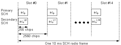
The Synchronisation Channel (SCH) is a downlink signal used for cell search. The SCH consists of two sub channels, the Primary and Secondary SCH. The 10 ms radio frames of the Primary and Secondary SCH are divided into 15 slots, each of length 2560 chips. Picture above illustrates the structure of the SCH radio frame.
The Primary SCH consists of a modulated code of length 256 chips, the primary synchronization code (PSC) is transmitted once every slot. The PSC is the same for every cell in the system.
The Secondary SCH consists of repeatedly transmitting a length 15 sequence of modulated codes of length 256 chips, the Secondary Synchronisation Codes (SSC), transmitted in parallel with the Primary SCH. The SSC is denoted csi,k in figure 20, where i = 0, 1, …, 63 is the number of the scrambling code group, and k = 0, 1, …, 14 is the slot number. Each SSC is chosen from a set of 16 different codes of length 256. This sequence on the Secondary SCH indicates which of the code groups the cell's downlink scrambling code belongs to.
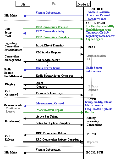
Summary of the process:
| Channel | Synchronisation acquired | Note |
| Primary SCH | Chip, Slot, Symbol Synchronisation | 256 chips The same in all cells |
| Secondary SCH | Frame Synchronisation, Code Group (one of 64) | 15-code sequence of secondary synchronisation codes. There are 16 secondary synchronisation codes. There are 64 S-SCH sequences corresponding to the 64 scrambling code groups 256 chips, different for different cells and slot intervals |
| Common Pilot CH | Scrambling code (one of 8) | To find the primary scrambling code from common pilot CH |
| PCCPCH *) | Super Frame Synchronisation, BCCH info | Fixed 30 kbps channel 27 kbps rate spreading factor 256 |
| SCCPCH **) | | Carries FACH and PCH channels Variable bit rate |
*) Primary Common Control Physical Channel
**) Secondary Common Control Physical Channel
Further reading: 3GPP TS 25.211 25.213
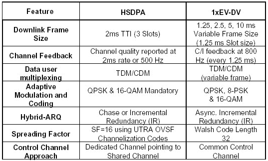
High Speed Downlink Packet Access (HSDPA) is a packet-based data service in W-CDMA downlink with data transmission up to 8-10 Mbps (and 20 Mbps for MIMO systems) over a 5MHz bandwidth in WCDMA downlink. HSDPA implementations includes Adaptive Modulation and Coding (AMC), Multiple-Input Multiple-Output (MIMO), Hybrid Automatic Request (HARQ), fast cell search, and advanced receiver design.
In 3rd generation partnership project (3GPP) standards, Release 4 specifications provide efficient IP support enabling provision of services through an all-IP core network and Release 5 specifications focus on HSDPA to provide data rates up to approximately 10 Mbps to support packet-based multimedia services. MIMO systems are the work item in Release 6 specifications, which will support even higher data transmission rates up to 20 Mbps. HSDPA is evolved from and backward compatible with Release 99 WCDMA systems.
Currently (2002) 3GPP is undertaking a feasibility study on high-speed downlink packet access.
 |
Further reading:
3GPP TS 25.855 High Speed Downlink Packet Access (HSDPA); Overall UTRAN description
3GPP TS 25.856 High Speed Downlink Packet Access (HSDPA); Layer 2 and 3 aspects
3GPP TS 25.876 Multiple-Input Multiple-Output Antenna Processing for HSDPA
3GPP TS 25.877 High Speed Downlink Packet Access (HSDPA) - Iub/Iur Protocol Aspects
3GPP TS 25.890 High Speed Downlink Packet Access (HSDPA); User Equipment (UE) radio transmission and reception (FDD)
 |
TDD WCDMA uses spreading factors 4 - 512 to spread the base band data over ~5MHz band. Spreading factor in dBs indicates the process gain. Spreading factor 128 = 21 dB process gain). Interference margin is calculated from that:
Interference Margin = Process Gain - (Required SNR + System Losses)
Overview of Spreading Process |
WiMAX Forum RF Network Engineer Certification Training Material Chapter 3, Antennas for WiMAX
0 comments Posted by communications at 7:37 PMAfter the first and second chapter of my self learning, here we go the third chapter ![]() titled Antennas for WiMAX. Just like traditional Wireless System, there are 3 kinds of antenna used for transceiving Radio Access Signal i.e., Omnidirectional, Sectoral, and Point to Point. The use of those antenna depends on it’s application.
titled Antennas for WiMAX. Just like traditional Wireless System, there are 3 kinds of antenna used for transceiving Radio Access Signal i.e., Omnidirectional, Sectoral, and Point to Point. The use of those antenna depends on it’s application.

1. Omnidirectional, broadcast 360 degree suitable for large area rural environment.

2. Sectoral, broadcast on intended area: 60, 90, and 120 degree. This kind of antenna is suitable for urban environment which has lage population on a certain area.

3. Point to Point Antenna is used for point to point communication, i.e., Microwave link, backbone etc.

(pictures are filched from wimax.com). If you need to read WiMAX Application material, please visit this my previous post, here
After we have discussed about those traditional antennas, now we are going to discuss advanced antenna technology in WiMAX.
1. Antenna Diversity,
Using two or more receiving antennas on a wireless device to eliminate multipath signal distortion. Typically, the signal from the antenna with the least noise (best SNR) is chosen, and the other antenna is ignored.
There are three techniques in diversity scheme:
1. Space Time Coding (Alamouti Code), is a method employed to improve the reliability of data transmission in wireless communication systems using multiple transmit antennas. STCs rely on transmitting multiple, redundantcopies of a data stream to the receiver in the hope that at least some of them may survive the physical pathbetween transmission and reception in a good enough state to allow reliable decoding. (resource: http://en.wikipedia.org/wiki/Space–time_code) Space time codes may be split into two main types:
- Space–time trellis codes (STTCs)[1] distribute a trellis codediversity gain. over multiple antennas and multiple time-slots and provide both coding gain and
- Space–time block codes (STBCs)[2][3] act on a block of data at once (similarly to block codes) and provide only diversity gain, but are much less complex in implementation terms than STTCs.


 .
.


